Concepts

Tasks

Settings

RBI Concepts

APM supports two types of risk analysis:

•	Failure mode risk analysis is performed on the failure mode as a whole

•	Demand scenario risk analysis is performed on each demand scenario identified for the failure mode

This topic explains each type and the concepts that are common to them. It also provides an overview of another central component of the RBI process: degradation (deterioration) tracking.

Failure Mode Risk Analysis

In the process of evaluating a failure mode, you can quantify the relative risk (criticality) associated with the failure by evaluating the consequences (severity of the effect), the probability of the failure occurring, and (optionally) the failure’s detectability, assigning values for each factor. APM then calculates the relative risk by multiplying the severity value by the probability value, and then by the detectability value, if it is used.

When the relative risk is established, APM calculates the failure mode’s consequence priority using a set of customer-defined rules. The consequence priority rules can be based on the failure mode’s severity, relative risk, downtime costs, downtime duration, or a combination. For example, the Extreme priority could be assigned to failure modes whose total severity is equal to 5.0.

After you have analyzed the failure modes, you can compare failure modes and identify the relative importance of addressing them. The Risk Assessment view in the Strategy Development Analysis window includes failure mode lists based on criticality, consequence priority, severity, and relative risk, as well as a risk plot, risk matrix, and lists of the evaluations. This view is also available for the asset.

APM provides two ways to perform failure mode risk analysis:

•	Using a simple evaluation that allows you to enter weighted severity values, probability values, and confidence factors

•	Using evaluation forms for in-depth analysis of consequences

With both methods, APM calculates the relative risk and displays it in the risk matrix chart. The method available in the Maintenance Action Plan window depends on the option selected in the analysis’ risk analysis settings.

Before you can perform risk analysis, the probabilities, severities, evaluation forms, consequence priorities, confidence factors, and risk matrix entries must be set up in the site’s RBI settings. For more information, see Setting up APM for RBI Analysis.

Demand Scenario Risk Analysis

APM provides a method of performing risk analysis on safety devices that protect equipment, people, and environments from events such as pressure build-up, fire, or equipment failure. Risk analysis is performed on one or more demand scenarios identified on the failure mode.

A demand scenario is a situation that requires that an asset, such as a safety device, be put into operation. Examples of demand scenarios are fire, power failure, and blocked outlet.

Probability Based on Likelihood of Failure and Demand Rate

When demand scenario analysis is performed, probability of failure is based on the likelihood of failure and demand rate. The analysis team determines the probability by:

•	Identifying the likelihood of the failure occurring based on past history or industry experience. This value describes how often the asset has been required to operate. An example of likelihood of failure is “Has happened at this location more than once in the last two years”.

•	Completing a confidence evaluation that quantifies the team’s faith in the current maintenance or inspection practices to contain the demand scenario’s risk. The confidence factor can adjust the likelihood of failure up or down.

•

Identifying one or more demand scenarios. These are the situations that result in the safety device being required. For each scenario, a demand rate is also selected. The demand rate is the frequency with which the scenario is likely to occur. Demand rates are typically defined in terms of 0-0.5 year, 0.5-1.0 year, and so on.

•	The demand rate with the highest criticality is used with the likelihood of failure to determine the probability of failure. APM uses the probability matrix to ascertain the result, and the selected probability of failure is added to the failure mode.

Demand Scenarios and the Failure Mode

The analysis team can then use questionnaires to evaluate the severity of consequences (health and safety, economic, environmental, reputation) to arrive at the demand scenario’s relative risk (criticality). APM uses the demand scenario with the highest criticality to represent the failure mode.

For information about setting up probability questionnaires and matrices, as well as likelihood of failure values, demand rates, and scenarios, see Failure Probability Settings.

The rest of this topic provides more detail about risk analysis concepts.

Risk (Criticality)

The risk number is calculated for the failure mode as the product of the Total failure mode severity, the probability of failure, and (optionally) the detectability of the failure.

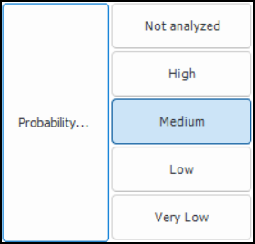
Risk = Severity * Probability * Detectability

Severity

Failure severity measures the consequences when a failure occurs. Severity can be described in terms of health and safety, environmental, reputation, and economic categories and is usually described as:

•

Severe

•

High

•

Medium

•

Low

•	Negligible

An impact statement and numerical value are associated with each severity value defined in APM. The higher the number, the more severe the effect. Economic impact can also be associated with each severity value to help determine avoidance savings and maintenance feasibility.

Probability of Failure

The probability of failure is the likelihood that the asset will fail due to the failure mode. There are three ways to evaluate probability:

•	Using a probability evaluation questionnaire

•	Based on the estimated time between failure

•	Based on the likelihood of failure and demand rate

Probability is usually described as high, medium, low, or negligible.

Detectability

“Detectability” refers to the ability of the system or process to detect a hazardous event. Lower scores are used for failures that are easy to detect and higher scores for failures that are harder to detect. When support for detectability is enabled in an analysis, the relative risk calculation becomes:

(Economic severity score + Health and safety severity score + Environmental severity score + Reputation severity score) * Probability score * Detectability score = Relative Risk Number

Consequences

For each important failure mode, the severity of the consequences of failure must be determined. Consequences are categorized:

•	Economic effects

•	Health and safety effects

•	Environmental effects

•	Reputation effects

Each of these consequence categories is assigned a value. The sum of the values in all categories is used in the calculation of the consequence assessment.

Economic Consequences

The economic consequence of failure reflects the financial effect of the failure on assets and production. Labor and material costs associated with lost production and with repairing or replacing the damaged equipment are economic consequences.

Costs associated with health or safety or environmental consequences are not included as economic consequences. For example, clean-up costs incurred as a result of a spill are not considered as an economic consequence.

Health and Safety Consequences

Equipment failure can cause hazards in the workplace. Examples are extreme temperatures or pressure or noxious fumes. It is important to note that mitigating factors are considered when assessing health and safety consequences:

•	The frequency of the hazard occurring and duration of exposure of people in the hazard zone

•	The possibility of averting the hazardous event

The following are examples of health and safety consequences:

Potential Impact	Description
No / slight injury	First aid or medical treatment, not affecting work performance or causing disability
Minor injury	Lost time injury affecting work performance such as modified work duties or time off work to recover
Major injury	Includes permanent partial disability, affecting long-term work performance. May include extended absence from work and damage to health such as chronic back injuries, sight or hearing loss.
Fatalities	May include single or multiple fatalities in close succession to the incident.

Environmental Consequences

Environmental incidents are an important category to consider when determining overall consequence. Typically, two types of environmental incidents are considered:

•	Release of liquids that may cause soil and water pollution

•	Release of gases that may cause atmospheric pollution

Several levels of consequence evaluation are taken into account, as shown in the table below:

Potential Impact	Description
No / slight effect	Local environmental damage, usually within the enclosed space or system. Negligible financial impact.
Minor effect	Contamination; damage sufficient to attack the environment. Typically a single complaint or single breach of statutory limits.
Localized effect	Limited loss of known toxic discharge but repeated breaches of statutory limits. Damage affects areas outside the enclosed space.
Major effect	Severe environmental damage. Extensive measures are required to restore the contaminated environment. Extended breach of statutory limits.
Severe effect	Persistent severe environmental damage or nuisance extending over a large area. A major loss to the organization in terms of commercial, recreational, or nature conservancy. Constant or extremely numerous breaches of statutory limits.

Reputation Consequences

Consequences to reputation measure the impact that negative media attention has on an organization’s ability to operate in good faith. Typically, the severity of bad press is evaluated in terms of how far-reaching it is and how long it takes to mitigate, as shown in the table below:

Potential Impact	Description
No / slight effect	Negative local press for less than a week
Minor effect	Negative provincial or state press for a week or more
Medium effect	Negative national press for a week or more
Major effect	Negative international press for a month
Severe effect	Negative international/national press for more than one month

Failure Mode Consequence Priority

APM calculates a consequence priority for the failure mode during risk analysis or for the failure during RCA evaluation. Consequence priorities allow you to rank and compare an asset’s failure modes and failures. In failure analysis, the consequence priority is used in the calculation that determines whether the failure is suitable for RCA.

The rules defined for a priority can be based on any of these properties:

•	Downtime cost – the total downtime cost of the failure mode or failure is used. The total downtime cost is the sum of the downtime occurrence cost and the downtime rate costs times the length of the downtime:

Downtime Cost = Downtime Occurrence Costs + (Downtime Rate * Downtime Duration)

•	Downtime duration

•	Failure cost

•	Relative risk (risk analysis only)

•	Severity, which can include the sum, minimum, or maximum value for any or all of:

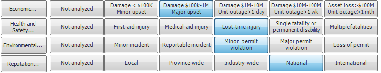
•	Health and safety consequences

•	Economic consequences

•	Environmental consequences

•	Reputation consequences

•	Failure mode consequences (risk analysis only)

The failure mode is assigned the highest ranking consequence priority for which it satisfies the priority’s rules.

As an example, suppose a set of three consequence priorities. To simplify the example, the rules are based on a single property (total severity). In practice, the rules can be more complex and involve multiple properties and rule groups.

Priority	Rank	Rule
High	3	Total severity is at least 12
Medium	2	Total severity is at least 6
Low	1	Total severity is at least 0

A failure mode with a severity of 14 is assigned the consequence priority High. Although it satisfies the rules for each of the consequence priorities, it is assigned High because that is the highest ranking priority.

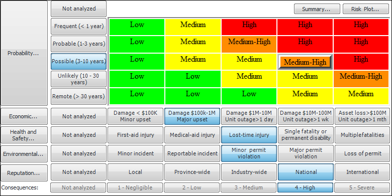
Risk Matrix

Criticality or risk is defined as the combination of two parameters: the likelihood or probability of failure and the consequences of failure. The risk matrix displays this combination, typically with four or five criticality levels and four or five probability levels. For example:

This example contains the following probability, consequence, priority, and criticality values.

Probability of Failure

Possible values are:

•	Frequent (<1 year) – Very High (5.00)

•	Probable (1-3 years) – High (4.00)

•	Possible (3-10 years) – Medium (3.00)

•	Unlikely (10-30 years) – Low(2.00)

•	Remote (> 30 years) – Very low (1.00)

Note: When the analysis supports detectability, the Detectability list is available below the risk matrix.

Consequence Categories

Possible values are:

•

Economic

•	Damage < $100K Minor upset (1.00)

•	Damage $100K Major upset (2.00)

•	Damage $1M-10M Unit outage (3.00)

•	Damage $10M-100M Unit outage >1 week (4.00)

•	Asset loss >$100M Unit outage >1 month (5.00)

•	Health and Safety

•	First-aid injury (1.00)

•	Medical-aid injury (2.00)

•	Lost-time injury (3.00)

•	Single fatality or permanent disability (4.00)

•	Multiple fatalities (5.00)

•	Environmental

•	Minor incident (1.0)

•	Reportable incident (2.0)

•	Minor permit violation (3.00)

•	Major permit violation (4.00)

•	Loss of permit (5.00)

•	Reputation

•	Local (1.0)

•	Province-wide (2.0)

•	Industry-wide (3.00)

•	National (4.00)

•	International (5.00)

Consequences

Possible values are:

•	Negligible – Any of (Environmental, Operational, Safety, Reputation) Is equal to 1.00

•	Low – Any of (Environmental, Operational, Safety, Reputation) Is equal to 2.00

•	Medium – Any of (Environmental, Operational, Safety, Reputation) Is equal to 3.00

•	High – Any of (Environmental, Operational, Safety, Reputation) Is equal to 4.00

•	Severe – Any of (Environmental, Operational, Safety, Reputation) Is at least 5.00

Criticality Rating

The criticality that is selected is the most severe combination of consequence priority and probability. For example, the Medium-high (MH) criticality is selected when the consequence priority is High and the probability of failure is Medium.

The ratings require corresponding responses. Negligible criticality can result in no formal inspection plan. Failure modes with low to medium-high criticalities usually require inspection plans. High and extreme criticalities can call for detailed analysis that can result in equipment redesign or further mitigating factors.

Confidence Factors

Confidence questionnaires are used to measure the analysis team’s faith in current maintenance or inspection practices to contain the failure mode’s risk. Confidence statements can include things like:

•	Is the equipment degradation mechanism stable and properly controlled?

•	Have multiple reliable inspections been performed?

•	Are the relevant process parameters reliably monitored?

The result of the evaluation is a confidence factor, which represents the analysis team’s faith in current maintenance or inspection practices to contain the failure mode’s risk. The confidence factor can adjust the inspection factor or likelihood of failure up or down.

An inspection factor is the portion of the asset’s remaining life calculated for the current degradation rate to be used when calculating indicator collection dates. For example, an inspection factor of “0.5” means that the indicator reading should be collected at half of remaining life. The greater the confidence factor, the higher the inspection factor, meaning that the interval between inspections is greater. The inspection factor is based on the confidence factor, degradation type, consequence priority (criticality), and (optionally) integrity group of the failure mode.

In some cases, typically when criticality is severe and confidence is low, an inspection strategy is recommended (for example, detailed analysis or redesign).

When risk assessment uses weighted severities, the confidence factor can adjust the location of a failure mode on the risk matrix. A negative confidence factor represents low confidence and moves the failure mode to the right on the consequence priority axis and up on the probability axis.

A positive confidence factor represents high confidence and moves the failure mode to the left on the consequence priority axis and down on the probability axis.

An adjustment value of 1 moves the failure mode one position on the matrix, a value of 2 moves it two positions, and so on.

For example, consider the results of the confidence factor on failure modes A and B:

•	Failure mode A is originally positioned at the Low Probability and Low Consequence Priority entry on the risk matrix. It has a confidence factor of Low, which has an adjustment value of -2.

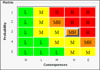
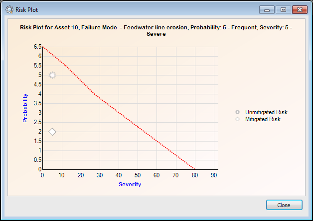
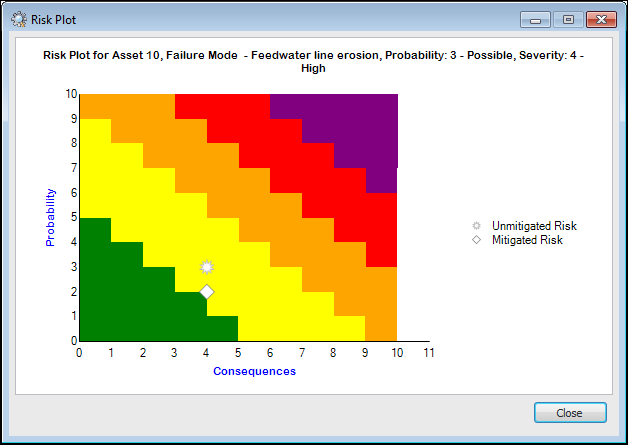
The failure mode is adjusted two positions to the right on the Consequence Priority axis and two positions up on the Probability axis, resulting in an adjusted risk matrix value of Extreme (represented by a1 in the following diagram).

•

Failure mode B is also positioned at Low/Low on the risk matrix. It has a confidence factor of High. High has an adjustment value of 1. The failure mode is adjusted one position to the left and down, resulting in an adjusted risk matrix value of Negligible (represented by b1 in the following diagram).

The following diagram shows how the confidence factor adjusts the positions of the two failure modes in the risk matrix:

Risk Plot Chart

Risk plot charts provide a visual representation of an asset’s unmitigated (or initial) risk based on severity (consequence) and probability of failure. The risk value is determined by asset prioritization or strategy development analysis. If a feasibility evaluation is performed on a failure mode, the chart also shows the mitigated (or residual) risk.

The risk plot chart can appear in the following locations:

•	Asset Prioritization Analysis window, Worksheet and Summary views

•	Maintenance Action Plan window, Criticality and Feasibility views (MTA2, RCM2, RBI analyses)

•	Strategy Development Analysis window, Risk Assessment view, Risk Plot tab

Risk plot lines indicate risk tolerance levels to provide context for analysis results. Tolerance levels can be shown as a single plot line or as color areas. Here is an example of a chart that shows a single risk plot line:

Risk plot charts support as many as five color areas (named Extreme, High, Medium, Low, Negligible). The default colors for the areas provided with APM are purple, red, orange, yellow, and green, respectively. Here is an example of a chart from a strategy development analysis:

Lookup Tables and Calculations

You can calculate the probability of failure and consequences for a failure mode based on various lookup tables and calculations to produce criticality evaluation rankings.

Note: Support for criticality evaluation calculations is generally available. However, you must first enable feature 115 to use the functionality in APM. In the Enterprise window, select the Features view and the Enabled Features tab. Click Browse, select “Practical RBI - criticality evaluation calculations” and click OK. If APM is running as a smart client, click Refresh Enabled Features on the server. Then restart the client to use the functionality.

The calculation function supports calculations that determine ranking values for criticality evaluations. In the criticality evaluation, the user is presented with a series of evaluation categories. Each evaluation category consists of a series of questions or impact statements.

Typically, the user would select the appropriate question for the failure mode being evaluated. The selected question has a ranking assigned to it. The ranking is used to select the corresponding probability or severity (health and safety, environmental, or reputation).

The ranking calculation provides an option to automate the determination of the ranking based on one or more inputs and the formula defined for the calculation. In most cases, the formula consists of a lookup table or a series of lookups. Once the ranking has been calculated, APM selects the corresponding question associated with the evaluation category.

In this example of a probability of failure evaluation, the user selected a degradation mechanism and entered the actual degradation rate. APM then determined:

1.	Degradation rate

2.

Ranking

3.	Lookup table used

4.	Probability question

5.	Probability

Asset Degradation Tracking

Degradation is the reduction in the ability of an asset to fulfill its intended purpose. This can be caused by various degradation mechanisms (for example, thinning, cracking, mechanical). Degradation tracking is the process of:

•	Recording the asset’s operating parameters, which provide information about the asset’s designed, actual, and integrity operating variables. Together, the operating parameters form the asset’s operating window, a framework of limits for the asset.

•	Creating indicators to track the asset’s operating parameters, record degradation over time, and calculate degradation rates.

•	Analyzing degradation information using strategy development analyses to estimate the probability and consequences of asset failure (risk), prioritize failure modes, and determine inspection intervals and strategies.

Degradation tracking is usually performed on assets that degrade at a measurable or predictable rate. It is most often used for age-related deterioration to determine the minimum value before replacement.

The asset type settings determine if degradation tracking can be performed for assets of that type.

 

Degradation Types

Degradation type describes the general nature of the asset’s deterioration. In APM, degradation type is used to determine the kind of confidence evaluation required. For RBI, three types of degradation are identified:

•	Age-related (AR)

•	Non-age-related (NAR)

•	Strategy-based (SB)

Age Related

•	Age-related degradation is stable and can be properly controlled. Age-related degradation is considered stable when it meets two conditions:

•	It remains constant over time

•	It does not change drastically with relatively small changes in process conditions

•	Multiple, reliable inspections have been carried out. In this context, multiple inspections are considered to be three or more. The inspections must have been reliable; the inspection method and locations must be adequate for detecting the degradation type that is being evaluated.

•

Relevant process parameters are reliably monitored. Typically, the corrosion engineer needs to determine which process parameters are relevant to the failure mode. These parameters can include temperature, flow velocity, concentration of corrosive materials, and so on. The process engineer needs to evaluate if the parameters are reliably and consistently monitored.

Non-Age Related

•	Degradation can be properly controlled. Degradation is not usually stable and can occur at any time. Control of non-age related degradation can be attained in two ways:

•	By selecting an adequate material that is resistant to the form of degradation

•	By changing the characteristics of the environment to make it less aggressive

•	Relevant process parameters are reliably monitored.

•	Reliable inspections have been carried out. Non-age related degradation is more likely to be monitored instead of inspected.

Strategy-Based

The selection of relevant strategies depends on criticality and confidence ratings.

Lining

Degradation type can also specify that assets with lining or coating require confidence evaluation and assign a questionnaire for that purpose.

Susceptibility to Failure Evaluation

Susceptibility to failure evaluation examines the asset’s non-age related degradation patterns. It can provide an alternative to probability of failure analysis for these failure modes. For example, susceptibility evaluation can be used to determine the vulnerability of atmospheric storage tanks to corrosion under insulation or stress cracking. The evaluation can result in recommended actions, susceptibility ratings, or both.

Degradation Patterns

The degradation pattern is the form that the general damage mechanism takes, for example, cracking or external pitting.

Degradation Mechanisms

A degradation mechanism is the type of deterioration that could lead to asset failure. Examples are corrosion, erosion, mechanical failure, and pitting.

Degradation Rates

Degradation rates are variable. The simplest method evaluates each inspection location independently and involves the following calculation:

previous thickness minus current thickness divided by the time between measurements

This degradation rate is then applied, using the remaining life equation above, to the actual thickness and minimum thickness at the point for which it was calculated, and the remaining life at that location is established. Because various locations can have different values for remaining life, the smallest remaining life is used for the entire equipment item, and the next inspection for that equipment item is set accordingly.

More advanced methods such as statistical analysis can also be used to establish the degradation rate. This is especially applicable for equipment or piping circuits that have large swings in corrosion rates. Often, a best-fit degradation rate is established over the entire circuit to each location. Because different points in the circuit can have different maximum wall thicknesses and possibly different minimum thicknesses, this produces a more conservative remaining life and therefore an earlier requirement for inspection.

Degradation Allowance

Degradation allowance is based on the maximum allowable wall loss. This value can be calculated by determining the difference between the minimum allowable wall thickness required to ensure integrity and the nominal or measured wall thickness.

Corrosion Loops

Corrosion loops are sometimes referred to as corrosion circuits. They provide a way to describe and control degradation mechanisms in sections of plants.

A corrosion loop is a section of a plant that:

•	Consists of similar materials of construction

•	Operates under similar process conditions

•	Is exposed to similar predicted degradation (corrosion) mechanisms, rates, and conditions

For example:

Remnant Life

The remnant life approach to determining inspection intervals is based on calculating the remaining life of the equipment or asset based on its tolerance to degradation, defects, or damage and the rate of degradation. The tolerance to degradation is determined by assessing the asset condition at future times according to the degradation predicted.

An inspection interval is defined as a percentage of the remaining life.

The remnant life calculation is based on the API 510/570 standard.

Integrity Operating Window

The integrity operating window is the normal operating condition required for the asset to perform.